How to Estimate Probability of Default for Credit Risk Models

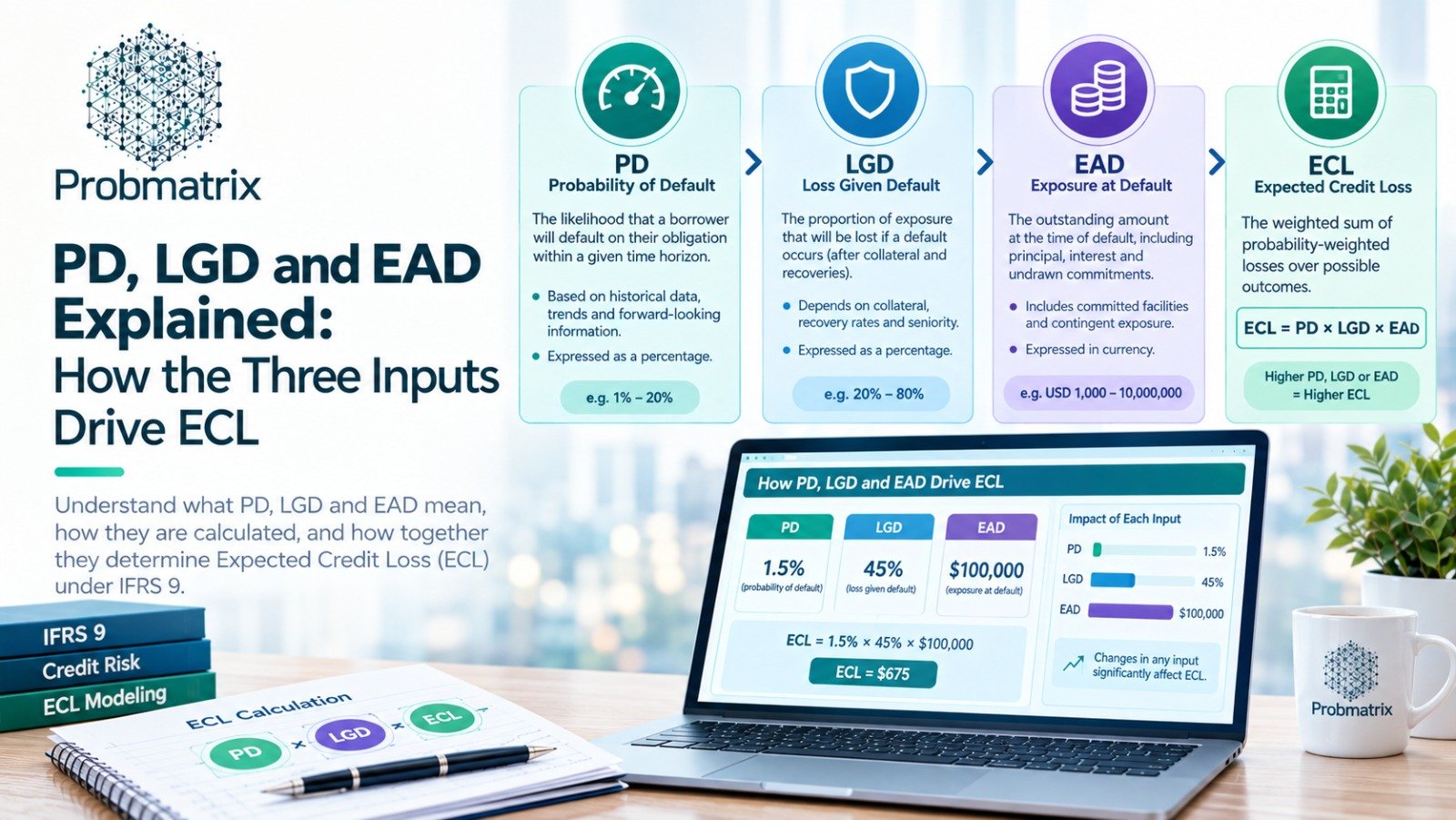
A probability of default model estimates the likelihood that a borrower or exposure will default over a defined period.

Under IFRS 9, PD is one of the core inputs used in Expected Credit Loss calculations, alongside LGD and EAD. A reliable IFRS 9 PD model should reflect both historical credit behavior and forward-looking economic conditions.

What Does a PD Model Measure?

A PD model answers a simple question:

What is the probability that this borrower will default within a given time horizon?

For Stage 1 exposures, the focus is generally on 12-month default risk. For Stage 2 exposures, the model needs to support lifetime PD estimation across the remaining life of the financial asset.

Common PD Modelling Methods

The appropriate PD modelling approach depends on the portfolio and the quality of available data.

Common methods include:

Observed Default Rate

The Observed Default Rate (ODR) methodology estimates PD using historical defaults by tracking performing customers over a defined performance window and measuring how many moves into default. It is generally considered a more conservative approach because it captures transitions into default but does not account for backward transitions or subsequent improvements in credit quality.

Roll-Rate Analysis

Roll-rate models track how exposures migrate through delinquency buckets, for example from current to 30 DPD, 60 DPD and ultimately default.

This method is commonly used for retail and other portfolios where detailed delinquency data is available.

Migration Matrix

A migration matrix tracks movements between credit-rating grades over time.

It can be particularly useful for corporate portfolios with established internal rating systems.

Pluto Tasche Low & Zero Default Models

The Pluto–Tasche approach is commonly used to estimate Probability of Default (PD) for low-default or zero-default portfolios, where historical default observations are insufficient for reliable empirical estimation. The method derives a statistically conservative PD by calculating an upper confidence bound on the default rate, based on the portfolio size, observed defaults, and selected confidence level. It is particularly useful for portfolios such as banks, sovereigns, large corporates, or other low-default segments, where limited default data can otherwise result in unrealistically low PD estimates.

From Historical PD to IFRS 9 PD

Historical default rates alone are usually not sufficient for an IFRS 9 PD model.

The model should reflect reasonable and supportable forward-looking information. This may require adjusting historical or through-the-cycle PD estimates using relevant macroeconomic variables.

Examples may include GDP growth, inflation, interest rates, unemployment or other portfolio-specific economic drivers.

Multiple economic scenarios may also be incorporated.

Probability of Default Calculation Example

Suppose 40 borrowers’ default during a year out of 1,000 performing borrowers at the start of the observation period.

A simplified probability of default calculation would be:

PD = 40 / 1,000 = 4%

However, this historical rate may still require calibration and forward-looking adjustment before being used in IFRS 9 ECL.

Key Takeaway

A strong probability of default model should do more than calculate a historical default percentage.

It should reflect the behavior of the portfolio, provide an appropriate PD term structure, respond to changing economic conditions and remain consistent with the institution’s definition of default.